Circuit Emulation in Software
Emulation of continuous-time systems can be broken into two distinct problems. First, a model must be constructed that characterizes the system suitably; second, a discrete-time implementation must be created that will faithfully represent the model. Depending on the system to be emulated, either the first or second part of the process can be the more challenging. We will treat the two parts separately here.
1. Construction of system model
Characterization of a system can theoretically be carried out in a number of ways. The two most widely used methods of system identification (system ID) are signal modeling and physical modeling. Signal modeling is the process of identifying a system based on its response to input signals, while physical modeling is study of a system based on a theoretical description of the system’s components. For systems whose inner workings are obscured from observation, signal modeling may be the only method of study available. If, however, something is known about the construction of a device, physical modeling can be used to improve our understanding of how that device will react to various input signals.
Signal Modeling
With signal modeling, a set of signals is applied to the system to be characterized, and the resulting outputs are measured (Fig. 1).

Depending on the nature of the system, the outputs from the test signals can be used to extrapolate how the system would respond to other input signals. Certain classes of systems can be completely characterized by a finite set of measurements. The most simple class of such systems is the Linear, Time-Invariant (LTI) System. Consider the system shown in Figure 1. We can denote N possible inputs to the system as xn(t) for 1 < n < N, and the corresponding outputs as yn(t). For example, if x1(t) is applied to this system, the output will be y1(t). If the system is LTI, then the output corresponding to input signal (αxn(t+τ1)+βxm(t+τ2)) will be (αyn(t+τ1)+βym(t+τ2)), for any xn(t) and xm(t).
"Program dependence is a feature whereby the release time of the compressor depends on the details of the signal being compressed."
In English, this means that we can mix multiple signals either before or after they have gone through the device, and get the same result. Examples of LTI systems include equalizers and many reverberators. LTI systems are convenient to study because their behavior can be fully characterized by a single measurement. In other words, one pair of input-output signals can be used to determine an LTI system's response to any signal. Most commonly, LTI systems are described by their response to an impulse signal. The impulse δ(t) is a signal whose value is equal to zero everywhere except at time zero, where the value of the signal approaches infinity. The impulse is thus a signal whose energy is entirely concentrated in a very short (infinitesimal) period of time. The response of the LTI system to the impulse signal is known as the system's impulse response. Through a process known as convolution, the impulse response can be used to calculate the response of an LTI system to any input signal.
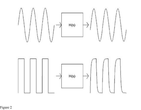
As an aside, LTI systems are systems for which exponential signals are eigenfunctions. A system's eigenfunctions are those functions which, when applied as inputs, are not distorted by the system. Rather, they are reproduced at the output of the system with some scaling and some time lag. When dealing with LTI systems, a convenient set of exponential functions to use as inputs is the set of sinusoids. When a sinusoid is applied as an input to an LTI system, the output will be an undistorted sinusoid at the same frequency as the input, with a possible scale factor and time delay. The scale factor corresponds to the amplitude response of the system, while the time delay corresponds to the phase response of the system. No matter what frequency sinusoid is applied to an LTI system, the output will always be an undistorted sinusoid at the same frequency. By contrast, if another type of signal, for example a square wave, is applied as an input to an LTI system, the output signal will not usually take the form of the input. Figure 2 shows responses of a lowpass filter (which is LTI) to a sine wave input and a square wave input. Notice that the sine wave input produces a sine wave output, but the square wave input produces an output of another shape.
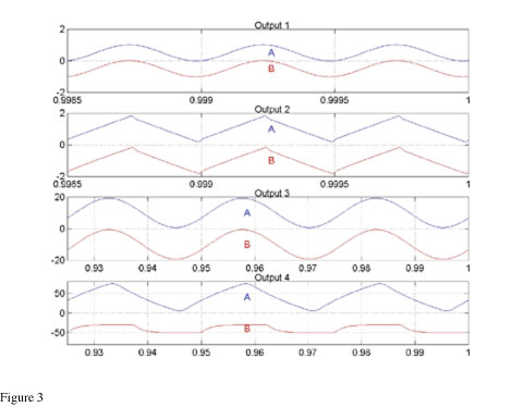
For systems that are not LTI, signal modeling becomes a more difficult task. The response of a non-LTI system to an unknown input signal cannot be calculated based on other, known, input-output pairs, no matter how much data is collected. This is illustrated in Figure 3. The figure shows responses for two systems, A and B, to four input signals. For the first three inputs, the responses of the two systems are indistinguishable. For the fourth input, the responses of the two systems are dramatically different. The first signal is a high-frequency sine-wave signal at low amplitude. At this level, the systems both appear to be linear, and to have the same gain and phase response. The second is a signal at the same frequency as the first signal, but at a higher level. Both systems seem to saturate in about the same way. The third is a low-frequency, low-level signal. Again, both systems appear linear, and have the same gain and phase response. The fourth is a signal at the same frequency as the third, but at a higher amplitude. As can be seen, at this frequency, the saturation properties of the two systems are not similar.
What is important about this example? It exposes a potential pitfall associated with signal modeling for non-LTI systems. If System B were a system being modeled, and only the first three signals were used to perform signal modeling, System A would appear to be a suitable model. However, if a user were to apply Signal 4 to the two systems, it would be apparent that System A was not a faithful model of System B.
In general, non-LTI systems cannot be characterized by signal modeling, because even if input-output signal relationships for N inputs xn(t) are known, the (N+1)th output signal cannot be predicted on the basis of the existing data. This is true even if N becomes very large.
Physical Modeling
Physical modeling is an attempt to characterize a system by understanding the processes that occur within the system. For electronic circuits, the understanding is usually arrived at by a combination of circuit theory and device physics. Rather than using input-output data to discover the behavior of a circuit, the structure of the circuit is analyzed in order to predict its behavior. Often, complex circuits can be broken up into subsystems whose behavior is relatively simple. System behavior is predicted by calculating how subsystems interact with one another. With physical modeling, input-output data can be used to calibrate system models to variations in component values within a circuit. Input-output data is also useful for recovering data that may not appear on a circuit's schematic, such as stray capacitances, leakage inductances, diode conduction curves, transistor beta values, et cetera. In many cases, particular input signals can be designed to expose circuit parameters that need to be measured. In some instances, it is difficult to measure some components in-circuit, and they may have to be removed from the circuit and characterized separately.

Figure 4 shows functional block diagrams for the two systems of Figure 3. It can be seen that the two systems have the same saturation mechanism followed by the same high-frequency filtering. But, the second system has additional low-frequency filtering before and after the nonlinearity. The functional diagrams of Figure 4 make it obvious how the systems differ. If the system in Figure 4 were modeled using physical modeling, the presence of the low-frequency filters would be known: Input signals could be specially created to expose the behavior of the low-frequency filters.
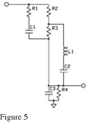
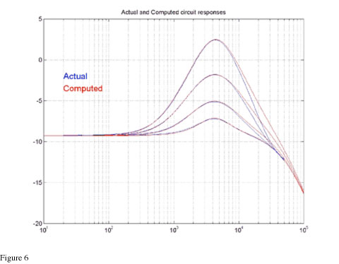
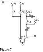
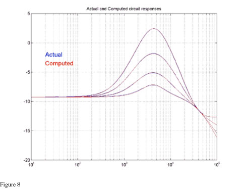
Figure 5 shows a schematic for a passive equalization filter. The frequency responses of the filter are plotted in Figure 6, along with the ideal responses for the circuit, as calculated from the schematic. As can be seen, the responses of the model do not match the actual behavior of the circuit. Figure 7 shows a modified schematic, which includes some parasitic effects associated with the components in the system. The response of this modified circuit is shown in Figure 8, along with data from the actual circuit. As can be seen, the model matches the data more closely with the inclusion of the parasitic effects. Note that the circuits in Figures 5 and 7 are both LTI systems, but the system in Figure 7 is a higher-order filter. Nonlinear effects can also be added to circuit models based on input-output behavior, as long as the mechanism for the nonlinearity is known.
We have seen that an LTI system can be effectively characterized by its impulse response, using signal modeling. However, this method can become cumbersome depending on how many controls the system has, and how those controls interact. For example, consider a linear equalizer that has a control with ten settings. For this system to be characterized using signal modeling, ten measurements would have to be made (one for each control setting). But what if the system has two controls, each with ten settings? In this case, if the control functions interact, there would be one hundred distinct system responses which would have to be measured in order to characterize the system. If there are four controls, 10,000 measurements would have to be made.
The problem becomes worse if one or more of the controls is continuously variable. In order to use signal modeling on a system with continuous controls, a decision must be made as to how far a control may be moved before the system response changes significantly. The sensitivity of a control may depend on the positions of the other controls, so that decision may not be trivial to make. If many measurements must be made, it may not be practical to store all of the required data within the system model. If one of the controls of the model is placed between the positions where data has been taken, the measured data must be interpolated to provide the desired system response.
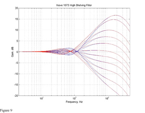
For all of these reasons, it may not be practical to use signal modeling even for some LTI systems. An example of a system whose controls interact is the Neve 1073. In the 1073, the high- and low-frequency equalization sections are implemented as active filters within the same gain stage. Figure 9 shows the high-frequency responses of the EQ with the low-frequency selector at "Off" (blue), and the same responses with the low-frequency selector at 220 Hz (red). Even though there is no low-frequency boost or cut being applied, the character of the high-shelving filter is influenced by the low-frequency selection. This behavior makes the high-filter more flexible, because different behavior can be coaxed out of it with different settings applied to the low-frequency selector. With signal modeling, much of this beautiful behavior could be missed. But if the system is studied using physical modeling techniques, interaction between controls will be automatically included in the system model.
For systems that are not LTI, it can be virtually impossible to perform system ID without some knowledge of system structure. Dynamic range control devices, in particular, are difficult to characterize on the basis of input-output relationships. Usually, the behavior of a dynamic-range compressor is represented by a static compression ratio, attack time, and release time. However, two different compressors can have identical ratios, attack times, and release times and behave in very different ways. Evidently, the common parameters used to describe a dynamic-range compressor do not fully characterize the system. Let us look at the behavior of the Universal Audio 1176 compressor in order to see how the actual behavior of a real-world device relates to the generic parameters used to characterize compression.
Usually, static compression curves are measured by recording the response of a compressor to a sinusoidal input at a single frequency. The input is held at constant amplitude until the output settles into steady state, and then the amplitude of the output is recorded. Output level is plotted as a function of input level, on a dB-dB scale. Static compression ratio is defined as the reciprocal of the slope of the static compression curve. For example, if an increase in input level of 4 dB results in an increase in output level of 1 dB, then the ratio of compression is 4:1.
The 1176 can be set to ratios of 4:1, 8:1, 12:1 and 20:1 using controls on the front panel. When the static compression curves are measured, the resulting ratios appear to be higher than the ratios prescribed by the controls. This is due to a property of the 1176 called program dependence. Program dependence is a feature whereby the release time of the compressor depends on the details of the signal being compressed. For signals whose peak levels are much higher than their RMS levels, the release time is relatively fast. For signals whose peak and RMS levels are comparable, the release time is slower. The motivation for program dependence is to prevent dropouts caused by gain reduction following heavy transients, while at the same time limiting distortion caused by gain modulation in low-frequency-rich signals. If the release time following a transient is short, the gain will be restored to nominal level as soon as possible. If the release time is relatively longer, the gain will modulate less for an input at a given frequency, reducing distortion.
As a side effect of the way the program dependence is implemented, the attack of the 1176 happens in two stages. The first stage of attack is fast, on the order of tens of microseconds. The second stage of the attack takes much longer. During the second stage of attack, the gain is reduced, causing the measured ratio of compression to go up. For signals whose time span is longer than the first attack stage, but shorter than the second, the effective compression ratio for the 1176 is close to what is prescribed by the controls of the unit. However, when compression ratios are measured using static sine waves, the second stage of attack is engaged, causing higher ratios to be observed.
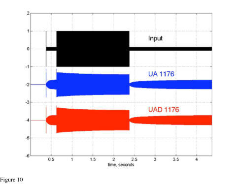
Program dependence affects the attack, release, and ratios of the 1176. Without a detailed model of how the 1176 accomplishes compression, it would be very difficult to make sense of input-output data. In fact, it would be very difficult even to know what input signals should be used to measure the behavior of the device. Figure 10 shows a signal created to expose the program-dependent behavior of the 1176. Figure 10 also shows the 1176 output for hardware and software emulation to this specially made signal. As can be seen, for both the hardware compressor and the model, the release following the transient at the beginning of the signal is faster than the release following the sustained high-amplitude portion of the signal.
2. Discrete-time implementation
After a suitable model of a continuous-time system has been created, the model must be implemented as a discrete-time system. The three most common problems in creating discrete-time emulations are (1) frequency warping due to transformations into discrete time, (2) aliasing caused by nonlinearities operating in discrete time, and (3) numerical difficulties. Frequency-warping problems are common when using the bilinear transform to map continuous-time filters onto the z-plane. The bilinear transform is convenient to use, because it preserves filter order and filter stability. With the bilinear transform, there is no aliasing of continuous-time frequency, but the continuous frequency axis is warped as it is being mapped onto the discrete-time frequency axis. Warping gets progressively worse at higher frequencies.
The simplest method for reduction of bilinear-induced warping is to use oversampling. Oversampling adds expense to algorithms, because the discrete-time filters must run at higher rates. Additionally, the resampling filters tend to be computationally expensive. However, oversampling minimizes frequency warping by placing the range of human hearing in a lower, and relatively less-warped, portion of the discrete-time spectrum. Oversampling is convenient, because the resampling filters can be designed independently of the filters to be discretized.
The problem of aliasing can also be addressed by oversampling. However, in the case of a system with nonlinearities, the resampling filters cannot be designed properly without knowing what kinds of nonlinearities are present. If a nonlinearity is static and can be represented by a power series, the bandwidth of the harmonics generated by the nonlinearity is finite, so that an anti-aliasing filter can always be designed to surpass any specification for aliasing rejection. However, higher sampling rates and better rejection require increased computational cost.
Numerical difficulties can arise for a number of reasons. Depending on the number system of the processor being used, the bit depth for data and coefficients, and the sampling rate, numerical problems can appear in different situations. In general, filters whose features lie at very low frequencies when compared to the sampling rate require higher numerical precision to achieve a given distortion floor. This can lead to great expense when oversampling, because the oversampled filters will need better precision in addition to running more often. Choice of filter structure influences numerical precision: for example, some lattice-filter structures have different pole locations for quantized coefficients than their direct-form counterparts. Lattice filters may also require smaller dynamic ranges for filter states, and can have a lower distortion floor for a given data bit-depth.
The most difficult combination of elements to implement in discrete time is a high-bandwidth nonlinearity within a feedback loop. For feedback systems containing frequency-dependent nonlinearities, it is necessary to solve numerically a nonlinear differential equation. If nonlinearities are significant, the solutions to the equation may have significantly more bandwidth than the input signal, so these solutions must be encoded at an increased sampling rate.
Summary
Modeling of systems can be carried out using signal analysis or physical modeling techniques. Physical modeling results in a more robust description of a system, and can lead to an improved selection of test signals to be used for calibrating the model.
No matter what modeling techniques are employed, implementation of system models must be carried out with care, and with an understanding of the limitations of discrete-time systems. When nonlinearities are present, special techniques must be used to ensure fidelity.
— Dr. Dave Berners
En lire plus
Tube Versus Solid-State Compressor Basics
Learn essential functions of popular tube and solid-state compressor varieties, and creative uses for your productions.
Recording Lyrics Born with Apollo’s Unison™ Technology
We chatted with Hamilton about his hybrid analog/digital recording studio, how he implements UAD plug-ins and Unison technology in his workflow, and the session he produced at at Studio G, his multi-room Brooklyn recording facility, tracking hip-hop artist Lyrics Born.
Tracking Arcade Fire With the Iconic UA 610 Console & Apollo
Learn how producer Steve Mackey (M.I.A., Florence and the Machine) used an original, and rare, Bill Putnam-designed UA 610 console — along with Apollo interfaces — on Arcade Fire's album, Everything Now.


